Project / Physics-informed neural networks
Right coefficients, wrong curve
I built a physics-informed neural network — a network trained on a differential equation instead of on examples of its solution — and pointed it at a damped harmonic oscillator, where I already knew every number it was supposed to find.
I gave the physics-informed neural network (PINN) twenty noisy measurements, no coefficients, and the single instruction that the system obeys $\ddot u + \mu\dot u + k u = 0$. It came back with $\mu = 3.923$ against a true 4, and $k = 401.2$ against a true 400 — closer on both than the classical least-squares fit I ran beside it, on the same twenty points. On every number I would have put in a paper, the network technically won.
Then I looked at the curve it drew to get there. Weight the physics term too lightly and the reconstruction walks out of phase: a stiffness three percent low, invisible across one oscillation and unmistakable across three. Tune the weighting until that seemingly disappears and something quieter is left behind. The error stops shrinking as the signal decays, so the reconstruction gets relatively worse exactly where the oscillator goes quiet. The network's curve drifts away from the exact solution of the equation it had just recovered. And the reconstruction has the oscillator moving at $\dot u(0) = 1.2$ when the real one was released from rest (i.e. it pulled out incorrect initial conditions).
The closer I looked, the more troubling the results appeared. For instance, whether the PINN reproduced reasonable results depended on the choice of weights that you would have no way of knowing unless you already knew the answer. Additionally, the curves PINN produced did things that a solution to the equations would not do, such as change phase mid oscillation.
What I take from this is that the coefficients and the solution are two separate deliverables, and a PINN can get one right while quietly getting the other wrong. Which of the two you actually need decides whether that matters — for a damping rate it does not, for a forecast or a reconstruction it is the whole story. The uncomfortable part is that I only caught it because I had an answer key. Every diagnostic the method offers from the inside — the loss curve, the physics residual, the agreement with the data — looked fine the entire time.
These are working notes, not a result. I am fairly sure about the measurements below and much less sure about what they mean. If you work with physics-informed neural networks and something here is wrong, or obvious, or already solved, I would like to hear it — reach out to me and let's talk.
Written September 2026. One test problem, one architecture; five seeds on the Case 2 weighting, one seed everywhere else.
What's in these notes
How a PINN works
Turning the equation into a cost function
A neural network is actually a differentiable function. Feed it $t$, get $u_\theta(t)$, and automatic differentiation hands you $\dot u_\theta$ and $\ddot u_\theta$ for free — exactly the derivatives the governing equation asks for. Substitute them into the equation and you get a residual you can evaluate anywhere you like:
Square it, average it over a scatter of sample points, and the differential equation has become a cost function. Drive that cost to zero and the network is a solution. No labelled examples, no training set of solved problems — the equation itself does the teaching. That is the whole trick, and it is a good one.
One cost function, three problems
The forward solve, data assimilation, and parameter estimation are not three algorithms, they are one objective with terms switched on and off.
The $t_i$ are wherever the measurements happened to land; the $t_j$ are collocation points, chosen freely, where the physics gets enforced. Switch $\lambda_{\text{data}}$ to zero and you have a solver. Turn it back on and you have a fit regularized by physics. Don't provide $\mu$ and $k$ and they become trainable, and you have system identification.
One bookkeeping detail, because it turns out to matter more than bookkeeping should. The residual in Eq. (1) carries the units of the equation, and here its terms run to $ku \sim 400$. Squared and averaged, that swamps a data term of order the noise. So every residual in this study is divided by a fixed $K_{\text{scale}} = 100$ before squaring. The constant is arbitrary and it is not free: it gets squared and absorbed straight into $\lambda_{\text{phys}}$, so a weight only means something once you say what you divided by. Every $\lambda$ below is quoted against that same $K_{\text{scale}} = 100$.
| Regime | $\lambda_{\text{data}}$ | $\lambda_{\text{phys}}$ | $\mu, k$ |
|---|---|---|---|
| Forward solve | 0 | > 0 | known, fixed |
| Data assimilation | > 0 | > 0 | known, fixed |
| Inverse / discovery | > 0 | > 0 | unknown, trainable |
In code the whole method fits on a screen. This is the inverse version, where mu_p and k_val() are trainable alongside the network weights:
def total_cost():
    # DATA: match the measurements
    cost = data_weight * torch.mean((net(t_data) - u_data) ** 2)

    # PHYSICS: residual of u'' + mu*u' + k*u, normalised by K_SCALE
    u    = net(t_phys)
    u_t  = torch.autograd.grad(u,   t_phys, torch.ones_like(u),   create_graph=True)[0]
    u_tt = torch.autograd.grad(u_t, t_phys, torch.ones_like(u_t), create_graph=True)[0]

    r = (u_tt + mu_p*u_t + k_val()*u) / K_SCALE

return cost + physics_weight * torch.mean(r ** 2)create_graph=True so the derivatives stay differentiable.What I ran
The test problem
To gain intuition and to put the PINN to the test, I chose a system we all know very well, a damped harmonic oscillator:
with $\mu = 2d$ and $k = \omega_0^2$. Underdamped, it decays into a sinusoid,
Throughout, the true parameters are $d = 2$ and $\omega_0 = 20$, so $\mu = 4$ and $k = 400$. Over $t \in [0,1]$ that is about three and a sixth oscillations, decaying to $e^{-2}$ — about an eighth of the starting amplitude — by the end of the window. Every claim below is graded against a fourth-order Runge–Kutta integration of Eq. (3) at $\Delta t = 10^{-4}$, and against the closed form in Eq. (4). The same Runge–Kutta solution generates the synthetic measurements.
The network throughout is a small fully connected stack with $\tanh$ activations — three hidden layers of 32 units for the problems with data, four of 64 for the forward solve — 2,209 parameters and 12,673. Smoothness is not a style preference here: the equation asks for $\ddot u_\theta$, and ReLU's second derivative is zero almost everywhere, so a ReLU network cannot represent this problem at all. It will train, report a falling loss, and hand you nothing.
Training runs in two stages, and since one of the results turns on the difference between them, both are worth naming. Adam is the workhorse optimizer of machine learning — gradient descent that keeps a running average of each weight's recent gradients and uses it to give that weight its own step size, so parameters with small or noisy gradients still move. It is cheap, robust, and knows nothing about curvature: it can only ever ask which way is downhill from where it stands. L-BFGS is the opposite bet. It is a quasi-Newton method that accumulates an approximation of the local curvature from the gradients it has already seen and uses it to jump most of the way to the bottom of the bowl in one step. That costs memory and needs to start somewhere sensible, but near a good solution it converges far faster than anything first-order can. Here the two run in sequence: Adam to get into the neighbourhood, L-BFGS to finish.
The three cases
Case 1 — solve the equation, no data. Set $\lambda_{\text{data}} = 0$. The network sees no solution values whatsoever, only 300 collocation points and the demand that Eq. (1) vanish at each of them. Fifty thousand Adam iterations, then two thousand of L-BFGS. The initial conditions go in by construction rather than by penalty:
which satisfies $u(0)=1$ and $\dot u(0)=0$ for every possible setting of the weights. It also closes off the escape route: $u \equiv 0$ solves Eq. (3) perfectly, and a network left to discover that on its own frequently will.
Case 2 — sparse data plus known physics. Fifteen measurements with Gaussian noise at $\sigma = 0.05$ and a deliberate gap: the sampler is forbidden to place a point in $t \in [0.45, 0.65]$, which leaves the record with no measurement at all between $t = 0.42$ and $t = 0.75$, with $\mu$ and $k$ held at their true values. Three competitors on identical data: a free-form network trained on the points alone ($\lambda_{\text{phys}} = 0$), the PINN with both terms live, and a classical least-squares fit of the known closed form in Eq. (4) — which, with $\mu$ known, has only the two linear amplitudes $A$ and $B$ left to find.
Case 3 — hide the coefficients. The one I actually care about. Throw away all knowledge of $\mu$ and $k$, keep only the form of the equation — a linear second-order system, coefficients unknown — and hand over twenty measurements at $\sigma = 0.05$. Both coefficients become trainable parameters sitting in the residual alongside the network weights, starting from deliberately wrong guesses ($\mu = 1$, $k = 100$).
For a fair fight, the same twenty points go to a classical estimator: fit Eq. (4) with $d$, $\omega$, $A$ and $B$ all free. Since $A$ and $B$ are linear once $d$ and $\omega$ are fixed, that reduces to a two-dimensional profiled search. Both methods get identical data and identical prior knowledge, and neither is told the initial conditions.
The weight sweeps
Equation (2) has two weights, and nothing in the method says what they should be. So two more experiments do nothing but vary them, re-training from the same seed at every setting.
On Case 3, $\lambda_{\text{data}}$ holds at 30 while $\lambda_{\text{phys}}$ walks 1, 30, 300, 3000, on one fixed set of twenty noisy points. The question is whether leaning harder on the physics buys a better answer, and how far you can lean before something breaks.
On Case 2, where $\mu$ and $k$ are known and a classical fit is available to grade against, $\lambda_{\text{data}}$ holds at 20 while $\lambda_{\text{phys}}$ walks five decades, and the settings get sorted into two piles: the ones a person could choose knowing nothing, and the one I picked by grading against the truth. That second pile is not a method that could be used a priori. It is used just to find the ceiling, and the gap between the piles is what not having an answer key costs. Then the same sweep runs again with the residual divided by 200, 400 and 300 instead of 100, to find out whether the best weight belongs to the problem or to that constant.
What came back
Solving from the equation alone (Case 1)
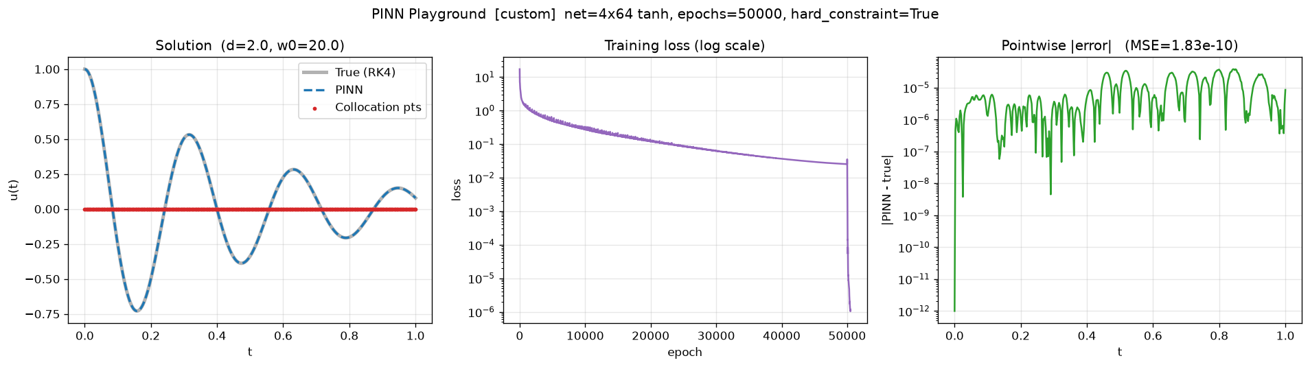
Two things came out of the forward solve (Figure 1) that I did not expect.
The first is that Adam does not get there. Fifty thousand iterations leave the solution sitting at $\mathrm{MSE} \approx 2\times10^{-3}$ against the Runge–Kutta reference, with the loss still visibly falling. Part of that is Adam being a first-order method on a badly conditioned problem, and part of it is spectral bias: smooth networks learn the low-frequency content first, and the low-frequency content of this solution is the decaying envelope. The three oscillations riding on top are precisely the part that comes last and comes hardest.
The second is what happens when you stop and switch optimizers. Two thousand iterations of L-BFGS take the error from $2\times10^{-3}$ to $1.8\times10^{-10}$. Seven orders of magnitude, from the last four percent of the training budget. On a smooth, low-dimensional problem like this one the Adam stage is not the heavy-hitter; it is the thing that gets L-BFGS into a basin where it can work its magic.
Do not read more than one digit into that $1.8\times10^{-10}$. The same script on a CPU lands between $5\times10^{-10}$ and $1.2\times10^{-9}$ depending on how many threads it is given — nothing changed but the order the floating-point sums are accumulated in. The seven orders of magnitude are the result; the specific number is just happenstance.
Adding data (Case 2)
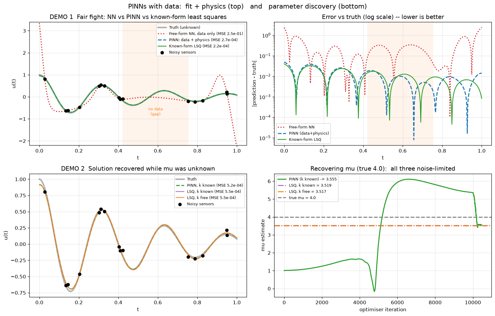
With fifteen noisy points and a gap in the middle, the free-form network does what free-form networks do (Figure 2, top): it goes through the measurements and invents structure everywhere else, filling the gap with confident nonsense and diverging the moment it runs out of data. It fits the measurements to an RMS of 0.008 — a sixth of the noise, so it is fitting the noise itself — and ends up at an MSE of $2.5\times10^{-1}$ against the truth.
Turn the physics term on and that becomes $2.7\times10^{-4}$. A factor of nine hundred, bought with no new data, just by enforcing the physics as well. The weights are $\lambda_{\text{data}} = \lambda_{\text{phys}} = 20$: equal, which is the obvious thing to write down when nothing tells you otherwise.
The least-squares fit still beats it, $2.2\times10^{-4}$ against $2.7\times10^{-4}$, with two parameters against the PINN's two thousand weights. The two curves are not the same curve, either: they differ by an RMS of 0.0061, an eighth of the noise, and by 31% of it where they diverge most. In RMS error that is 0.0147 for least squares against 0.0165 for the PINN — each about a third of the $\sigma = 0.05$ noise on a single measurement, with the PINN's twelve percent larger.
Twelve percent sounds like something to brush off as an accident of this particular data set, but I do not think it is. On five independent draws of the noise the classical fit wins four. The size of the win wanders; the direction mostly does not. Something systematic is going on, and it is not that networks are bad at drawing curves.
With $\mu$ and $k$ pinned at their true values, the functions satisfying Eq. (3) are exactly the two-parameter family of Eq. (4) — the same family the least-squares fit searches. Enforce the equation exactly and “find the curve that best matches the data while solving the ODE” stops being a rival method. It is basically least squares, written a different way, with the same minimum. So an exact tie is what a PINN ought to score here, whatever the noise did. Anything else means the network is not solving the problem the equation poses.
It does not tie, and the difference is the part worth having. $\lambda_{\text{phys}}$ is finite, which makes the equation a preference rather than a requirement. And the residual is enforced at a few hundred collocation points rather than everywhere — driving $r(t_j)$ to zero at each $t_j$ leaves two thousand weights free to do as they please between them. Soften the constraint and the network stops solving the least-squares problem and starts solving one close to it. Graded against the truth that neither method sees, that neighbouring problem usually does worse — by seven to twenty-five percent on three of the five draws, more than four times over on the fifth. But, not always. On the fourth draw it lands nine percent closer to the truth than least squares, by the luck of where the noise fell.
The bottom half of Figure 2 runs a second experiment: the same fifteen points, $k$ held at truth, $\mu$ turned loose. The network lands on $\mu = 3.56$ and the classical estimator on $3.52$, against a true 4. It gets there by a strange route — the estimate creeps from 1 to 1.6 over four thousand iterations, dips below zero (negative damping, an oscillator that would gain energy), shoots past 6, and is still above 5 when Adam finishes; L-BFGS hauls it back to 3.56 in its last few hundred evaluations — but it arrives. Both are about a ninth low, and the network's curve is marginally the better of the two. Neither method is losing to the other here. Both are losing to fifteen points with a hole in the middle.
What if I change the weights?
Hold everything else fixed — the same fifteen points, $\lambda_{\text{data}} = 20$ — and walk $\lambda_{\text{phys}}$ across five decades.
| $\lambda_{\text{phys}}$ | Solution MSE | In the gap | × LSQ | What happened |
|---|---|---|---|---|
| 0.0625 | 3.8 × 10⁻³ | 9.8 × 10⁻³ | 17.4 | as I first wrote it |
| 0.6 | 5.9 × 10⁻⁴ | 6.1 × 10⁻⁴ | 2.72 | |
| 2 | 4.0 × 10⁻⁴ | 1.5 × 10⁻⁴ | 1.86 | |
| 6 | 3.2 × 10⁻⁴ | 7.4 × 10⁻⁵ | 1.47 | |
| 20 | 2.7 × 10⁻⁴ | 8.5 × 10⁻⁵ | 1.25 | equal weights |
| 30 | 2.4 × 10⁻⁴ | 7.9 × 10⁻⁵ | 1.12 | |
| 40 | 2.3 × 10⁻⁴ | 7.8 × 10⁻⁵ | 1.07 | |
| 50 | 2.3 × 10⁻⁴ | 8.0 × 10⁻⁵ | 1.06 | best in the scan |
| 60 | 4.9 × 10⁻⁴ | 2.6 × 10⁻⁴ | 2.25 | coming apart |
| 80 | 1.3 × 10⁻¹ | 5.5 × 10⁻² | 593 | collapse to $u \equiv 0$ |
| Known-form LSQ | 2.2 × 10⁻⁴ | 1.1 × 10⁻⁴ | 1.0 | two parameters |
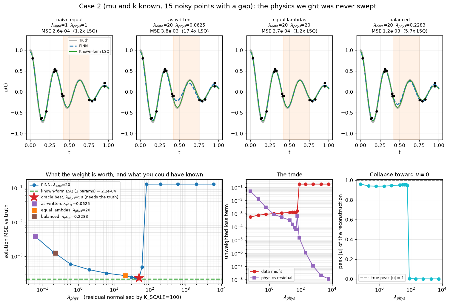
The top row is what I first ran: no physics weight typed at all, in a script that divided the residual by 400 rather than 100, which works out to 0.0625 here and 17 times the classical error. Equal weights reaches $2.7\times10^{-4}$ against the classical $2.2\times10^{-4}$. It is not the best row. Lean harder on the physics and the error keeps falling, to $2.3\times10^{-4}$ at 50 — and one step further the whole thing comes apart: 60 doubles the error, and 80 collapses onto $u \equiv 0$ (Figure 3, bottom left). Inside the gap, where the equation carries the curve alone, every setting from 6 to 50 beats the closed form by twenty to thirty percent.
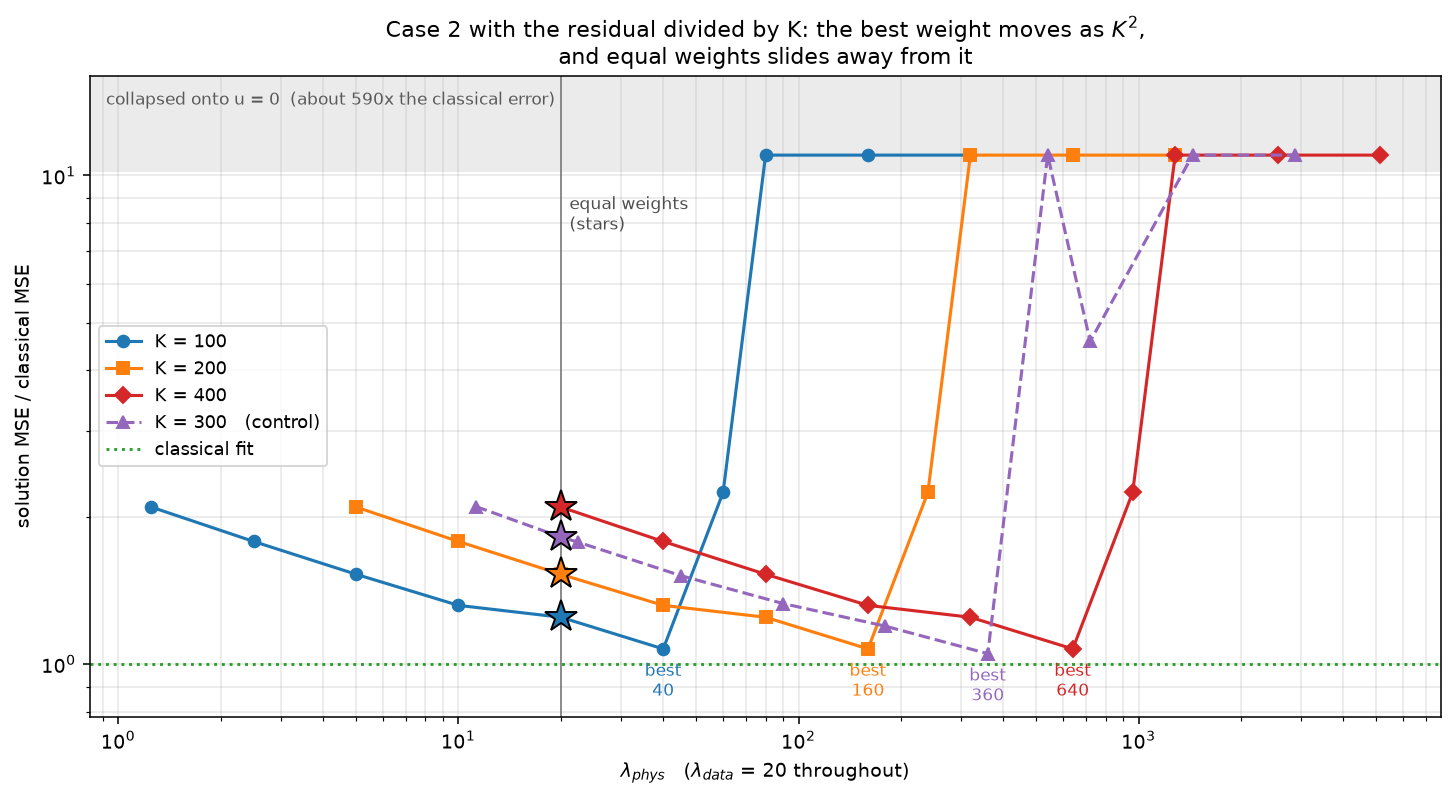
Equal weights looks like the obvious default, but the equality depends on a constant I didn't choose for the purpose. Whatever the residual is divided by gets squared into the weight, and this study used two. The Case 2 script divided by $k$, which makes the $ku$ term exactly the size of $u$ — possible only because $k$ is known here. The inverse scripts cannot know $k$, so they divide by 100, an order-of-magnitude guess put there to precondition the optimizer, and when I made every script agree, that guess became the standard. Neither was chosen with this sweep in hand.
So I ran the sweep again with the residual divided by 200, by 400, and — as a control — by 300 (Figure 4). Only $\lambda_{\text{phys}}/K_{\text{scale}}^2$ ever reaches the optimizer, and it shows. Divide by 200 and every run is the same run, bit for bit, as dividing by 100 with a quarter of the weight; divide by 400 and it is the run with a sixteenth. On a grid that doubles the weight at each step, the best moves from 40 to 160 to 640 — exactly the square of the constant. Equal weights stays at 20 and slides away from it: 1.25 times the classical error at 100, 1.53 at 200, and 2.10 at 400, the constant the Case 2 script actually used. The control at 300 lands within a few percent of the others away from the collapse, because dividing by three is not exact in binary and the rounding compounds over eleven thousand steps. Next to the collapse, the rounding decides: at 300 the network collapses at a weight the other constants survive, and survives the next weight up, where the others collapse.
An approach to dealing with this that came to mind that needs no answer key: make the two terms equal, not the two weights. But this actually did worse. Train once, read off both terms at the end, and set the physics weight so its term matches the data term. In the run I first did, the physics term was a quarter the size of the data term, so the rule raises $\lambda_{\text{phys}}$ from 0.0625 to 0.23. That lands at 5.7 times the classical error, worse than equal weights (Figure 3, top right). The rule takes its answer from that one trial run. The trial run barely enforced the equation, so its residual was large, and a large residual needs only a small weight to match. Start the trial run at the best weight, 50, and the same rule asks for 416, far past the collapse.
Across five seeds:
| $\lambda_{\text{phys}}$ | 1 | 2 | 3 | 4 | 5 | median |
|---|---|---|---|---|---|---|
| 0.0625 | 17.4 | 27.5 | 13.6 | 8.85 | 253 | 17.4 |
| 1.25 | 2.10 | 4.88 | 2.32 | 1.50 | 36.2 | 2.32 |
| 6.25 | 1.43 | 1.99 | 1.25 | 1.06 | 10.7 | 1.43 |
| 20 | 1.25 | 1.17 | 1.07 | 0.91 | 4.44 | 1.17 |
| 30 | 1.12 | 1.06 | 1.04 | 0.93 | 3.18 | 1.06 |
| 40 | 1.07 | 5.17 | 1.03 | 0.79 | 3.35 | 1.07 |
| 50 | 1.06 | 2.25 | 1.04 | 0.60 | 3.21 | 1.06 |
| 60 | 2.25 | 1246 | 1.09 | 0.52 | 4.60 | 2.25 |
| 80 | 593 | 1247 | 1.06 | 0.63 | 99.0 | 99.0 |
Equal weights is not the best setting on any seed. The best settings sit at 30, 30, 40, 50 and 60, and across seeds the median is flat at about 1.06 from 30 to 50. The 1.25 row is equal weights under $k = 400$; its median of 2.32, against 1.17 at 20, is what the constant was worth.
The bottom rows are the warning. Each seed's best sits close to a cliff, and the cliff moves. Seed 2 does best at 30; at 40 it is five times the classical error, and at 60 it has collapsed onto $u \equiv 0$ — peak amplitude 0.003, where the truth starts at 1. Seed 4 does best at 60, which gives the best single run in the study, at half the classical error. Same weight, a different draw of the same noise: one run is the best answer available and the next is a flat line. On a CPU the cliff moves again, and seed 1 collapses at 60 as well. And the collapsed runs carry the smallest physics residual in the scan (Figure 3, bottom middle).
So: tuned against an answer key, the PINN lands within six percent of the classical fit. Equal weights, the obvious guess, lands twenty-five percent behind it here — and would have landed at twice the classical error had the constant been 400. Run the way I first ran it, it loses by a factor of seventeen. A normalization constant and a weight I never typed account for the whole gap, and nothing in the loss, the residual or the fit to the data said so. This goes to show that the weights, and the constant they are scaled against, are part of the result: a PINN number reported without them cannot be checked, even by the person who ran it.
Hiding the coefficients
With both coefficients unknown, the PINN and the classical estimator land in nearly the same place (Figure 5).
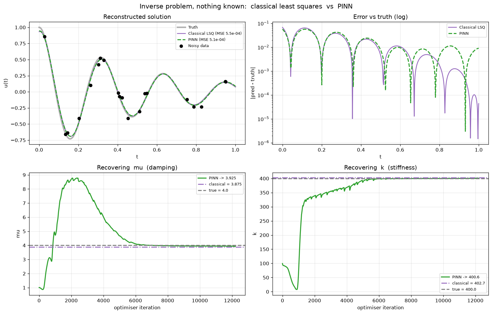
| Method | $\mu$ | $k$ | Solution MSE |
|---|---|---|---|
| Classical least squares | 3.875 (−3.13%) | 402.71 (+0.68%) | 5.49 × 10⁻⁴ |
| PINN | 3.925 (−1.87%) | 400.61 (+0.15%) | 5.10 × 10⁻⁴ |
Both methods land inside the noise. Neither is meaningfully better than the other.
The agreement is not luck. Once the data have pinned the solution down, demanding $\ddot u_\theta + \mu\dot u_\theta + k u_\theta \approx 0$ is nothing more than estimating the coefficients of a linear relationship between $\ddot u_\theta$ and the pair $(\dot u_\theta, u_\theta)$. The classical method runs that regression in the exact analytical basis. The PINN runs the same regression in a basis it invented. Same identification problem, different scaffolding.
So: parameter estimation, excellent. That is where I almost stopped, and that would have been a trap!
Where the phase slip comes from
Lean too hard on the data and not hard enough on the physics and something strange happens. The reconstruction goes through every measurement. The early oscillations lie on top of the truth. Then a peak arrives late, and every peak after it is wrong (Figure 6, left).
This isn't just getting the coefficients wrong, it's worse. A frequency error accumulates. The lag it produces is $\delta\omega \cdot t$ — proportional to elapsed time, always the same sign, never recovering. So measure the lag directly. Find every zero crossing of the network's curve, find the matching crossing of the truth, and difference them.
| Crossing at $t \approx$ | 0.08 | 0.24 | 0.40 | 0.56 | 0.72 | 0.87 |
|---|---|---|---|---|---|---|
| Measured lag | +0.2° | +5.6° | +3.6° | −5.5° | +8.4° | +19.3° |
| If it were a frequency error | +1.4° | +4.2° | +6.9° | +9.6° | +12.3° | +15.0° |
Read the two rows against each other (plotted in the middle panel of Figure 6). The network is running slow, so a frequency error predicts a lag that is late everywhere and climbs steadily: $+1.4^\circ$ to $+15^\circ$, one sign, straight line. What the curve actually does is drift late, come back, cross zero, go negative — at $t = 0.56$ the network arrives early — and then jump to nearly twenty degrees behind. It wanders. No frequency error can do that, because $\delta\omega \cdot t$ cannot change sign while $\delta\omega$ is fixed.
So put the question the strongest way I know. Forget the recovered coefficients; take the network's curve on its own terms and ask whether any damped oscillator could have produced it. Fit Eq. (4) to the network's own output — not to the data, to the curve — with $d$, $\omega$, $A$ and $B$ all free. That is the closest the entire solution family can get to what the network drew.
It reaches $d = 1.852$, $\omega = 19.758$, and still misses by an RMS of $2.8\times10^{-2}$. For scale, the true solution misses the network's curve by $3.6\times10^{-2}$. The best member of the whole family is barely better at describing that curve than the right answer is.
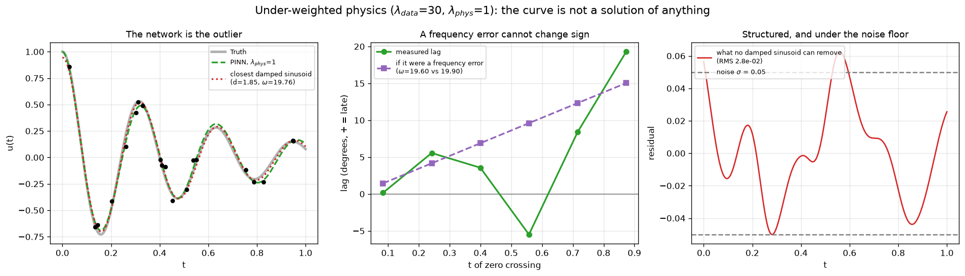
Which means the curve is not the right solution carrying the wrong coefficients. It is not a solution at all. There is no $\mu$, no $k$, no pair of amplitudes that produces it. The network has drawn something that locally resembles a damped oscillation and globally is not one.
Put that way the mechanism is not mysterious, and it is worse than a bad parameter estimate. A functional solution has a single $\omega$ governing every cycle: the closed form ties the phase at $t = 0.9$ to the phase at $t = 0.1$ whether you want it to or not. The network has no such tie. It has two thousand weights fitting whatever is nearby and 200 collocation points carrying a residual penalty I had turned down almost to nothing. Nothing in that arrangement carries a constraint from one end of the record to the other. Each stretch of curve is free to be locally plausible and globally incoherent — which is exactly what a lag that drifts, reverses and then jumps looks like.
And the recovered $k = 388$ is not the cause of any of it. It is a symptom. It is the answer to a question nobody meant to ask: given this curve, which is not an oscillator solution, what coefficients come closest to making it satisfy the equation? The causality runs the opposite way from the story I first told myself.
What makes it hard to catch is in the right panel of Figure 6. The leftover — the part of the network's curve that no damped sinusoid can account for — is smooth and clearly structured, plainly not noise. And it sits at an RMS of $2.8\times10^{-2}$, comfortably beneath the $\sigma = 0.05$ noise on the measurements. A structural failure, hiding under the noise floor. The cost function was perfectly happy. The data term was small. Nothing in the training history says anything is wrong.
The best I could do
Raising the physics weight from 1 to 30 does what it should (Figure 7): $k$ climbs to 401.2, the phase drift closes up, and the solution error drops by a factor of two and a half.
Push further and the whole thing comes apart, in a way worth staring at. Equation (3) is homogeneous. It has a trivial solution. Weight the physics term at 3000 and the network finds it — the reconstruction goes flat, $k$ collapses to 91.7, and the solution error is the worst in the sweep — 250 times the balanced setting's.
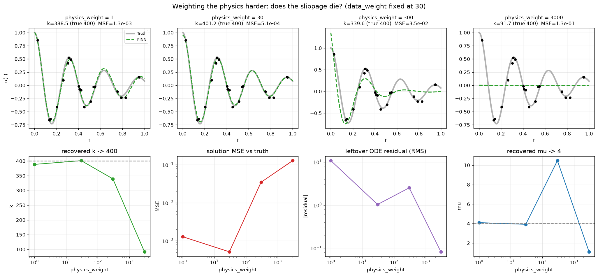
| $\lambda_{\text{phys}}$ | Recovered $k$ | Solution MSE | What happened |
|---|---|---|---|
| 1 | 388.5 | 1.3 × 10⁻³ | Under-weighted — phase slip |
| 30 | 401.2 | 5.1 × 10⁻⁴ | Balanced |
| 300 | 339.6 | 3.5 × 10⁻² | Over-weighted — the fit degrades |
| 3000 | 91.7 | 1.3 × 10⁻¹ | Collapse toward $u \equiv 0$ |
Now look at the leftover residual, the third panel along the bottom of Figure 7. At $\lambda_{\text{phys}} = 3000$ it is the smallest anywhere in the sweep. The run that satisfies the differential equation better than any other run is the run that learned nothing. A flat line obeys the physics beautifully.
I cannot think of a cleaner demonstration that the physics residual is not a quality metric. It is a constraint, and constraints are satisfiable in ways you did not intend.
What I think it means
What survives at the best setting
Take the best setting from the sweep — $\lambda_{\text{data}} = \lambda_{\text{phys}} = 30$ — and look hard at what it produced.
| $\mu$ | $k$ | $\omega$ (true 19.900) | Solution MSE | |
|---|---|---|---|---|
| PINN | 3.923 (−1.93%) | 401.23 (+0.31%) | 19.934 | 5.12 × 10⁻⁴ |
| Classical least squares | 3.879 (−3.03%) | 402.85 (+0.71%) | 19.977 | 5.49 × 10⁻⁴ |
Every headline number says the PINN won. A stiffness three tenths of a percent high against the classical fit's seven. A recovered frequency closer to the truth. A lower solution MSE. If this were a report or paper, that is the table that would go in it, and the phase slip would be a paragraph in the past tense about an earlier version.
Here is what that table hides (Figure 8).
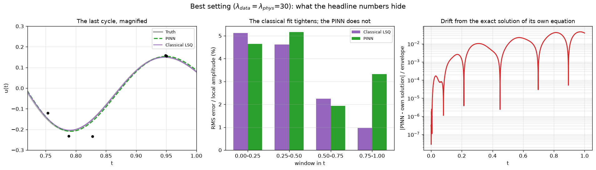
The error stops shrinking with the signal. The oscillation decays to about an eighth of its starting amplitude across the window, so a fixed absolute error means a steadily worse relative one. Splitting the record into quarters and taking the RMS error against the local envelope (plotted in the middle panel of Figure 8):
| Window | Classical LSQ | PINN |
|---|---|---|
| $t \in [0.00, 0.25]$ | 5.1% | 4.6% |
| $t \in [0.25, 0.50]$ | 4.6% | 5.2% |
| $t \in [0.50, 0.75]$ | 2.2% | 1.9% |
| $t \in [0.75, 1.00]$ | 1.0% | 3.3% |
The classical fit tightens by a factor of five across the record. The PINN manages one and a half. Averaged over the whole window — which is what MSE does — the two are indistinguishable, because MSE on a decaying signal is dominated by the loud beginning and says almost nothing about the quiet end.
The network does not solve its own equation. This is the one I keep coming back to. Take the recovered $\mu = 3.923$ and $k = 401.23$, take the network's own value and slope at $t = 0$, and integrate that initial-value problem with a real solver. Compare the result to the curve the network actually drew. They separate, monotonically, from $0.14\%$ of the envelope in the first quarter to $3.3\%$ in the last (Figure 8, right).
That is not a phase slip in the earlier sense — the recovered frequency here is essentially exact. It is the network carrying a small equation residual and letting it accumulate. The leftover residual has RMS 1.0 against terms whose own RMS is 139, three quarters of one percent. Small, and enough. The coefficients are excellent; the function is not quite a solution of the equation those coefficients define.
The reconstruction starts the oscillator wrong. The network reports $u(0) = 0.942$ and $\dot u(0) = 1.198$. The real system was released from rest. Nothing in the inverse setup told the network otherwise — the initial conditions are not given, and there is no hard constraint like Eq. (5) holding it — so this is not cheating so much as an unforced choice nobody was checking. But the reconstruction claims the mass was thrown when in fact it was dropped, it costs essentially nothing in the cost function, and it is completely invisible in $\mu$ and $k$.
That last one is the general shape of the worry. The optimizer will spend anything it is not being charged for. If the only quantities under scrutiny are the two coefficients, then everything else — the shape between data points, the implied initial state, the accumulated residual — is currency the optimizer can spend to make those two coefficients look good. And it will.
Does it matter that the curve is wrong?
The honest answer is that it depends entirely on what you asked for.
If you wanted the coefficients — a damping rate, a diffusivity, a reaction constant, a material property you are going to quote — then the PINN mysteriously delivered, and the defects in the reconstruction cost you nothing. The curve was scaffolding. You can throw it away. However, how would you even begin to think about putting an uncertainty bar on this value?
If you wanted a forecast — where is this system at $t = 10$ — then the accumulated drift is the whole story and the coefficients are cold comfort. Better to take the recovered coefficients and integrate them properly with a solver you trust, which costs microseconds and has error bounds somebody has proven.
If you wanted the reconstruction itself — the field between the sensors, the flow between measurement planes, the state where you could not put a probe — then the curve is the deliverable. However, saying "but the parameters are accurate" is not at all a reasonable defense for using PINN to fill in the gaps.
What makes me uneasy is not that the method has a failure mode. Everything has a failure mode. It is that this particular failure mode is silent, and that the window between the two ways of failing — too little physics gives you a wrong $k$, too much gives you $u \equiv 0$ — was found by sweeping a weight against a truth I possessed. In a real problem I would not possess it. I would have had one run, one number for $k$, a loss curve that went down, and no reason to look further.
What I would check without an answer key
So what is left to check when you cannot plot against the truth? Here is my current list. I do not think it is complete, and it is the part I would most like to argue with someone about.
- Integrate your own recovered equation and compare. Take $\hat\mu$, $\hat k$, and the network's own initial state, hand them to a conventional solver, and difference the two curves. This needs no truth, costs nothing, and is what exposed the drift in Figure 8. If a PINN's output disagrees with the exact solution of the PINN's own equation, at least one of them is not what you think it is.
- Scale the residual against the terms, not against zero. A residual RMS of 1.0 sounds terrible or wonderful depending on whether $ku$ is of order 1 or of order 400. Report the ratio.
- Measure error relative to the local signal, not globally. MSE over a decaying, growing, or intermittent signal reports on whichever part is loudest. Normalize by a local amplitude and the quiet regions get a vote.
- Check the implied state against what you actually know. The initial conditions, the boundary values, a conserved quantity, a symmetry, a sign. Anything you did not put in the cost function is a free check on whether the solution is physical.
- Sweep the weight and watch whether the parameters move. If $k$ slides across a decade of $\lambda_{\text{phys}}$ while the total loss barely changes, the data are not determining $k$ — the weighting is. That is a red flag you can raise without knowing the answer.
- Re-run it. Then run it on another machine. Then run it twice in a row. All three found something here. Move the identical script to a CPU and $k$ becomes 400.73, the free-form baseline changes by a factor of two, and seed 1 collapses at a weight the GPU survives. Run it twice in the same process and the first run disagrees with every one after it, because the first pass through the GPU happens before its linear-algebra library has a context and takes a different path to the same sum. That reaches the good settings too, not just the fragile ones: equal weights in Case 2 moves by two percent in one script and eight in another, depending on what each had done first. So every number on this page now comes from runs that throw away a few optimizer steps first. None of that is physics, and one piece of it had already crept into the prose: run cold, the Case 2 PINN looked fifteen percent worse than least squares; warm, it is twenty-five.
Open questions I have not resolved, in rough order of how much they bother me:
- Is there a principled way to set $\lambda_{\text{phys}}$ without a truth to sweep against? There is literature on adaptive and self-balancing weights; I have not tested any of it here, and I would like to know what actually works in practice.
- Should the residual be normalized term by term rather than by a single constant? Here $\ddot u$, $\mu \dot u$, and $ku$ differ in magnitude, and a single $K_{\text{scale}}$ weights the equation's own terms against each other by accident.
- When the initial conditions are known, should they always go in as a hard constraint even in the inverse problem? Equation (5) costs nothing and removes an entire family of wrong answers. I did not do this, and I am not sure why not.
- Is the residual drift a property of PINNs, or of this optimizer, this architecture, this problem, this seed? I have one of each. That is not enough to say anything general, and I am aware that the strongest-sounding sentences above rest on it.
Should I use PINN or a classical method?
None of the above is an argument against the method. It is an argument about where the method is worth reaching for, which sorts itself by how much you know before you start.
If the solution form is known, use it. Fit Eq. (4) with four parameters and go home. The damped oscillator lives here, which is exactly why classical least squares matches the PINN at every stage of this study while using four numbers instead of two thousand weights. A neural representation buys flexibility, and flexibility is not accuracy.
A known form does not have to be a closed form. With $d$ and $\omega$ fixed, Eq. (4) is a basis of two functions. A spectral basis — Fourier modes, Chebyshev polynomials — can hold thousands, and least squares fits their coefficients the same way, to problems no closed form describes. In my Ph.D. thesis I fit a spectral expansion to low-Reynolds-number turbulence data: nonlinear, high-dimensional, and on no structured grid at all (Crowley 2022, §3.3.3). Each coefficient still owns one mode of the answer. I expect a fit like that to match or beat a PINN for the same reason Eq. (4) does here, though I have not tested it.
If the equation is known but the solution is not, you are in PINN territory — and also in the territory of every conventional solver ever written, which is worth remembering. The equation supplies the information that a labelled dataset would otherwise have to. When is PINN better than a conventional solver? I do not know.
If no governing model is known, you are back to free-form machine learning, which will want far more data and will extrapolate badly. Case 2 (Figure 2) shows that middle ground cleanly: the physics term is what stops a network from inventing structure in the gap.
A hard problem, then, is not automatically a PINN problem. Nonlinear dynamics, a high-dimensional state and scattered data do not rule out a structured fit; my thesis data had all three. What a PINN offers instead is freedom from choosing a basis. Some problems make that choice hard: a geometry too irregular for a global basis, or so many independent variables that the basis cannot be stored — ten modes along each of twenty axes is already $10^{20}$ coefficients. That is where not needing a basis is worth something, and it is exactly where the failure above stops being interesting and starts being dangerous: the harder a basis is to build, the less there is to check a PINN against. Where a basis can be built, fit it first. A PINN that cannot beat that fit has not earned its keep.
Losing the structure
Everything above rests on something worth saying plainly. I could only see any of it because I already had the answer.
I noticed the phase slip by drawing the reconstruction on top of a curve I had generated myself. I found the working weight by sweeping $\lambda_{\text{phys}}$ and keeping the value whose error against that same known curve was smallest. I established that the network drifts off its own equation by integrating a system whose coefficients I had chosen in the first place. Take the answer key away and not one of those three steps survives.
So ask the questions in the order they would actually arrive. How would I know to look for a phase slip at all? Nothing announces it — the cost falls, the residual is small, the curve goes through the data. How would I set the weights? The sweep that produced $k = 401.2$ also produced $k = 91.7$, and the only thing separating the good run from the collapsed one is a comparison I could not have made. And having set them, how would I check the result?
The obvious escape is held-out data: fit on some points, test on the others. It does not work here, and the numbers say why. In the slipping run the reconstruction sits at $\mathrm{MSE} = 1.3\times10^{-3}$ against the truth while the measurement noise carries a variance of $2.5\times10^{-3}$. The wrong curve is closer to the truth than the measurements are. No held-out point can flag a discrepancy smaller than the noise you would be measuring it with — and that is precisely where the slip lives. It is not a large error. It is a small error pointed in a direction that accumulates.
What is actually missing is a relationship the classical fit gave me for free. Write the solution as $u = e^{-dt}(A\cos\omega t + B\sin\omega t)$ and the error structure is legible on the page. $\omega$ owns the phase, and an error in it grows linearly in $t$. $d$ owns the envelope. $A$ and $B$ own where the thing started. Each parameter is responsible for a specific feature of the answer, so when something comes back wrong I know what it should have looked like if it were right, and I know which parameter to suspect.
A PINN dissolves that. $\mu$ and $k$ are two scalars bolted onto a residual; the solution is two thousand weights bearing no interpretable relation to either. The coefficients no longer own any part of the curve. There is no expression in which a small $\omega$ error visibly becomes a growing phase error — the error simply happens, spread across the weights, with nothing to be inconsistent with. That is why the failure is silent. Not because it is subtle, but because there is no structure left for it to violate.
And that is the trade I do not think gets discussed enough. We give up the functional form in order to handle problems that have no functional form. But the functional form was never only a way to compute the answer — it was the thing that carried our intuition about how the answer behaves. Surrender it and both go at once, in the same move. Whatever is supposed to replace it has to be a check rigorous enough to certify a solution from the outside, because the inside has stopped telling us anything.
So here is the claim, and I think it is stronger than it first sounds. A PINN can recover the coefficients of a system more accurately than a classical fit and still be drawing a curve that is not a solution of the equation it just found. Those two facts are not in tension; that is simply what a soft constraint means. But nothing inside the method separates the two cases, and nothing outside it did either until I checked against an answer I had no business having. Until we have a way to establish that a PINN's output is feasible without already knowing that output, I do not think we are entitled to trust one — not because the method is wrong, but because being careful with it is not yet something we know how to do.
The code
Every script behind these notes is at github.com/cjcrowley/pinn-damped-oscillator, along with every number and figure they produced and what it takes to run them yourself.
References
- C. J. Crowley, “Evidence for the dynamical relevance of relative periodic orbits in turbulence,” Ph.D. thesis, Georgia Institute of Technology (2022). hdl:1853/67187 — Chapter 3; the spectral fit is in §3.3.3.