Resource
Notes on curve fitting
Least squares, total least squares, and how to pull a defensible uncertainty out of a calibration fit.
Every calibration I've done ends at the same place: a cloud of points, a model, and the question of how much to trust the curve drawn through them. Fitting the curve is the easy part — a one-liner in any language. The uncertainty on that curve is where the work is, and it's the part most fitting routines hand back either wrong or not at all.
These are the notes I keep for that. They start from the linear least-squares problem, extend it to the case where the x values carry uncertainty too, and end with the pieces you actually report: a fit band, a reduced chi-squared, and a single number for the calibration. Along the way, three worked examples — what "linear in the parameters" really means, a thermistor calibrated against the Steinhart–Hart model, and a flowmeter calibrated against another flowmeter.
You don't have to build any of this yourself. Everything derived here is implemented and working, in MATLAB and in Python, and the code is yours to take. Both versions build the design matrix from a model string you write the way you'd write it on paper, and hand back the whole uncertainty budget — not just the coefficients. Section 4 documents the interface.
Written January 2025, updated March 2026.
What's in these notes
1 Least squares when the model is linear in $\vec{\beta}$
1.1 Ordinary least squares
Given a model $f(x_i;\vec{\beta})$, build a model matrix — a design matrix — that captures the functional form, so that
where $\vec{\mathcal{E}}$ is the error.
If
$$f(x;\vec{\beta}) = a_0 + a_1 x + a_2 x^2 + \cos\left(2\pi x\right)$$
then
$$\mathbf{X}=\begin{bmatrix} 1 & x_1 & x_1^2 & \cos\left(2\pi x_1\right)\\ 1 & x_2 & x_2^2 & \cos\left(2\pi x_2\right)\\ \vdots & \vdots & \vdots & \vdots\\ 1 & x_N & x_N^2 & \cos\left(2\pi x_N\right) \end{bmatrix}$$
and
$$\vec{\beta}=\begin{bmatrix} a_0 \\ a_1 \\ a_2 \\ 1 \end{bmatrix}$$
such that
$$f(x;\vec{\beta}) = \mathbf{X}\vec{\beta} + \vec{\mathcal{E}}.$$
The $\cos\left(2\pi x\right)$ term is wildly nonlinear in $x$, and it doesn't matter at all. What matters is that every parameter enters the model multiplied by something that depends only on the data.
Writing the problem in matrix form, and ignoring the error term for the moment, it looks like
To find the optimal solution, find the projection of $\vec{y}$ onto the column space of $\mathbf{X}$. That is, project the data onto the basis spanned by the functional form.
Write $\vec{y}$ as
$$\vec{y} = \mathbf{P}_{\!x}\vec{y} + \left(\vec{y}-\mathbf{P}_{\!x}\vec{y}\right),$$
where $\mathbf{P}_{\!x}\vec{y}$ is the projection of $\vec{y}$ onto the column space of $\mathbf{X}$. The residual vector $\left(\vec{y}-\mathbf{P}_{\!x}\vec{y}\right)$ is orthogonal to that column space, and therefore
$$\mathbf{X}^\mathsf{T}\left(\vec{y}-\mathbf{P}_{\!x}\vec{y}\right)=\vec{0}.$$
Since $\mathbf{P}_{\!x}\vec{y}=\mathbf{X}\hat{\vec{\beta}}$ — where $\hat{\vec{\beta}}$ denotes the estimate of the true parameter vector $\vec{\beta}$ computed from the data — this gives
$$\mathbf{X}^\mathsf{T}\vec{y} = \mathbf{X}^\mathsf{T}\mathbf{X}\hat{\vec{\beta}},$$
which are the normal equations.
If the columns of $\mathbf{X}$ are linearly independent, then $\mathbf{X}^\mathsf{T}\mathbf{X}$ is invertible and the optimal coefficients follow:
To get the covariance of the estimator $\hat{\vec{\beta}}$, go back to the model in (1.1) and substitute it into (1.3):
$$\begin{aligned} \hat{\vec{\beta}} &=\left(\mathbf{X}^\mathsf{T}\mathbf{X}\right)^{-1}\mathbf{X}^\mathsf{T}\left(\mathbf{X}\vec{\beta}+\vec{\mathcal{E}}\right) \\ &=\vec{\beta}+\left(\mathbf{X}^\mathsf{T}\mathbf{X}\right)^{-1}\mathbf{X}^\mathsf{T}\vec{\mathcal{E}}. \end{aligned}$$
Take the covariance — $\vec{\beta}$ is deterministic, so it drops out — and use the identity $\mathrm{Cov}(\mathbf{A}\vec{X})=\mathbf{A}\,\mathrm{Cov}(\vec{X})\,\mathbf{A}^\mathsf{T}$:
Assume $\mathrm{Cov}(\vec{\mathcal{E}})=\sigma^2\mathbf{I}$ — independent, homoscedastic errors — and (1.4) collapses to
If instead each data point has its own variance and the errors are uncorrelated, $\mathrm{Cov}(\vec{\mathcal{E}})$ is diagonal but not proportional to the identity, and the covariance stays in the general form of (1.4).
1.2 Weighted least squares
The weighted residual sum of squares is
where $w_i$ is the weight of the $i^\mathrm{th}$ data point and $\mathbf{W}=\mathrm{diag}(w_1,\dots,w_N)$. The second equality assumes $f(x_i;\vec{\beta})$ is linear in the parameters, so that it can be written $\mathbf{X}\vec{\beta}$.
Minimizing (1.6) with respect to $\vec{\beta}$ gives the normal equations
$$\mathbf{X}^\mathsf{T}\mathbf{W}\mathbf{X}\hat{\vec{\beta}} = \mathbf{X}^\mathsf{T}\mathbf{W}\vec{y},$$
with solution
Substituting the model $\vec{y}=\mathbf{X}\vec{\beta}+\vec{\mathcal{E}}$ into (1.7) and taking the covariance, exactly as before, gives
Weighting is just a rescaling
Weighted least squares is ordinary least squares on rescaled variables. That matters practically: if you already have a routine that returns parameter estimates and covariances for the unweighted problem, you can get the weighted answer by rescaling the data and the design matrix and calling the same routine.
Define scaled variables
$$\vec{y}^{\,\prime}=\mathbf{W}^{1/2}\vec{y}, \qquad \mathbf{X}'=\mathbf{W}^{1/2}\mathbf{X}.$$
Then the ordinary residual sum of squares for the transformed variables is
$$\begin{aligned} \mathrm{RSS}' &= \left(\vec{y}^{\,\prime}-\mathbf{X}'\vec{\beta}\right)^\mathsf{T}\left(\vec{y}^{\,\prime}-\mathbf{X}'\vec{\beta}\right) \\[4pt] &= \left(\mathbf{W}^{1/2}\left(\vec{y}-\mathbf{X}\vec{\beta}\right)\right)^\mathsf{T}\left(\mathbf{W}^{1/2}\left(\vec{y}-\mathbf{X}\vec{\beta}\right)\right) \\[4pt] &= \left(\vec{y}-\mathbf{X}\vec{\beta}\right)^\mathsf{T}\mathbf{W}^{1/2\,\mathsf{T}}\mathbf{W}^{1/2}\left(\vec{y}-\mathbf{X}\vec{\beta}\right) \\[4pt] &= \left(\vec{y}-\mathbf{X}\vec{\beta}\right)^\mathsf{T}\mathbf{W}\left(\vec{y}-\mathbf{X}\vec{\beta}\right) \;=\; \mathrm{WRSS}. \end{aligned}$$
So weighted least squares is ordinary least squares applied to the transformed model $\vec{y}^{\,\prime}=\mathbf{X}'\vec{\beta}+\vec{\mathcal{E}}^{\,\prime}$, with $\vec{\mathcal{E}}^{\,\prime}=\mathbf{W}^{1/2}\vec{\mathcal{E}}$. The covariance follows directly from the unweighted formula applied to $\mathbf{X}'$.
If the weights are inverse variances
If the measurement errors are uncorrelated with known variances $\sigma_i^2$, then $\mathrm{Cov}(\vec{\mathcal{E}}) = \mathbf{\Sigma} = \mathrm{diag}(\sigma_1^2,\dots,\sigma_N^2)$, and choosing
$$\mathbf{W} = \mathbf{\Sigma}^{-1} = \mathrm{diag}\!\left(\frac{1}{\sigma_1^2},\dots,\frac{1}{\sigma_N^2}\right)$$
simplifies (1.8) to
Unknown overall variance scale
If only relative weights are known, compute $\hat{\vec{\beta}}$ from (1.7), then the weighted residual sum of squares
$$\mathrm{WRSS} = \left(\vec{y}-\mathbf{X}\hat{\vec{\beta}}\right)^\mathsf{T}\mathbf{W}\left(\vec{y}-\mathbf{X}\hat{\vec{\beta}}\right),$$
and estimate the variance factor
$$\hat{\sigma}^2 = \frac{\mathrm{WRSS}}{N-p},$$
where $p$ is the number of fitted parameters. The covariance is then
Take the calibration of a negative-temperature-coefficient thermistor. The procedure gives measurements of resistance $R$ in ohms and temperature $T$ in kelvin, each carrying its own uncertainty, $u_{R_i}$ and $u_{T_i}$.
The Steinhart–Hart model
$$\frac{1}{T} = A + B \ln R + D \left(\ln R\right)^3$$
relates resistance to temperature. It doesn't look linear in the parameters until you define
$$y = \frac{1}{T}, \qquad x = \ln R,$$
which turns the model into
$$y = A + B x + D x^3,$$
with design matrix
$$\mathbf{X}=\begin{bmatrix} 1 & x_1 & x_1^3 \\ 1 & x_2 & x_2^3 \\ \vdots & \vdots & \vdots \\ 1 & x_N & x_N^3 \end{bmatrix}, \qquad \vec{\beta}=\begin{bmatrix} A \\ B \\ D \end{bmatrix},$$
so that $f(x;\vec{\beta}) = \mathbf{X}\vec{\beta} + \vec{\mathcal{E}}$.
To run a weighted fit, you need $w_i=u^{-2}_{i}$, and that $u_i$ has to capture the uncertainty in each data point going into the fit — meaning it has to account for both $u_{R_i}$ and $u_{T_i}$. The obvious route is propagation of uncertainty:
$$\begin{aligned} u^2_{y_i} &= \left(\frac{\partial y_i}{\partial T_i}u_{T_i}\right)^2 + \left(\frac{\partial y_i}{\partial R_i}u_{R_i}\right)^2\\[4pt] &= \left(\frac{u_{T_i}}{T^2_i}\right)^2 + \left(\frac{B+3D\left(\ln R_i\right)^2}{R_i}u_{R_i}\right)^2. \end{aligned}$$
Look at what that requires: $B$ and $D$, which are the output of the fit and not known in advance. The circularity is handled naturally by the iterative total least squares of Section 2.1 — at each iteration the current estimate of $\vec{\beta}$ sets the effective variances, which in turn update the estimate.
Alternatives, if a full TLS implementation isn't available
- Iterative reweighting. Run an unweighted fit to get initial estimates of $B$ and $D$, compute $\sigma_{\mathrm{eff},i}^2$, then run a weighted fit. Repeat until it converges.
- Ignore one uncertainty. If $u_{R,i} \ll u_{T,i}$, or the reverse, treat the smaller as negligible and use standard weighted least squares. This underestimates the total uncertainty in $\hat{\vec{\beta}}$.
2 Fits with uncertainty in both $x_i$ and $y_i$
The methods in Sections 1.1 and 1.2 put all the measurement uncertainty in the dependent variable $\vec{y}$ and treat the independent variables in $\mathbf{X}$ as known exactly. In most physical measurements that's false: both carry error. This class of problem goes by several names — errors-in-variables regression, orthogonal regression, total least squares. For the single-parameter case with a constant variance ratio, the classical solution is Deming regression. What follows generalizes to multiple parameters with observation-specific uncertainties in every measured quantity.
2.1 Total least squares
Start from the underlying physical relationship
where "true" denotes the unknown error-free values. The measurements are corrupted versions of these:
with the measurement uncertainties independent and normally distributed:
Maximum-likelihood formulation
Under those assumptions, the joint probability density of the observed data given the true values is
Take the negative logarithm and drop the constants:
Define corrections $\delta y_i = y_{\mathrm{true},i} - y_i = -\epsilon_{y,i}$ and $\delta X_{ij} = X_{\mathrm{true},ij} - X_{ij} = -\epsilon_{X,ij}$. The maximum-likelihood estimates come from minimizing
subject to the constraint that the corrected data satisfy the model exactly:
Geometric interpretation
Each row of the augmented matrix $\mathbf{A} = \begin{bmatrix} \mathbf{X} & \vec{y} \end{bmatrix}$ is a measured point in $(p+1)$-dimensional space, and the model $\vec{y} = \mathbf{X}\vec{\beta}$ is a $p$-dimensional hyperplane through the origin. Ordinary least squares minimizes the vertical distance from each point to that hyperplane — the right thing to do when only $\vec{y}$ carries error. Total least squares minimizes the orthogonal distance, treating every coordinate as uncertain. The weights $1/\sigma^2$ scale each coordinate by its precision, stretching the space so a unit displacement in any direction is one standard deviation of measurement error.
Solution methods
When every measurement shares a common variance ($\sigma_{y,i} = \sigma_{X,ij} = \sigma$ for all $i,j$), the problem reduces to finding the hyperplane that minimizes orthogonal distances in an isotropic sense, and a singular value decomposition of the augmented matrix $\mathbf{A}$ gives a closed-form answer.
When the uncertainties differ between coordinates or between observations, there is no closed form. The problem becomes a nonlinear optimization solved iteratively. Two approaches are common:
- Iterative reweighting. Alternate between estimating $\vec{\beta}$ by weighted least squares — treating the current $\delta\mathbf{X}$ estimates as known — and updating the corrections $\delta\vec{y}$, $\delta\mathbf{X}$ given the current $\vec{\beta}$.
- Direct optimization. Minimize (2.6) with a standard nonlinear solver such as Levenberg–Marquardt, treating both $\vec{\beta}$ and the corrections as unknowns.
Covariance of the TLS estimator
Unlike ordinary least squares, the TLS estimator $\hat{\vec{\beta}}$ has no explicit formula in terms of the data — it's defined as the solution to an optimization problem. To get its covariance, ask instead: if the measured data were slightly different, how much would $\hat{\vec{\beta}}$ move?
At the solution, define the corrected design matrix $\hat{\mathbf{X}} = \mathbf{X} + \delta\mathbf{X}$ and an effective variance for each observation. That effective variance captures how uncertainty in every measured quantity propagates into the residual $r_i = y_i - \sum_j X_{ij}\beta_j$. For uncorrelated measurement errors, standard propagation of uncertainty gives
Each $x$-uncertainty enters through its sensitivity coefficient $\partial r_i / \partial X_{ij} = -\beta_j$, so $\beta_j^2$ converts $X_{ij}$-uncertainty into equivalent $y$-uncertainty.
When quantities within an observation are correlated, the full covariance form is needed. Let $\vec{z}_i = [X_{i1}, \ldots, X_{ip},\, y_i]^\mathsf{T}$ be the vector of measured quantities for observation $i$, with covariance matrix $\mathbf{\Sigma}_{z,i}$. The sensitivity vector is
and propagation of uncertainty gives
Expanded, that is
which reduces to (2.8) when the covariances vanish.
Either way, linearizing the residuals gives the covariance of $\hat{\vec{\beta}}$ to first order:
where
Note that (2.12) has the same structure as the weighted least-squares covariance $(\mathbf{X}^\mathsf{T}\mathbf{W}\mathbf{X})^{-1}$, with two changes: the corrected design matrix $\hat{\mathbf{X}}$ replaces $\mathbf{X}$, and the effective weights carry uncertainty from every measured variable. This is a first-order approximation — for problems with large relative uncertainties, Monte Carlo or bootstrap methods give more reliable estimates.
Calibrate a flowmeter against a reference standard. Both the reference flow rate $x_i$ and the meter reading $y_i$ carry measurement uncertainty, $u_{x,i}$ and $u_{y,i}$. The calibration model is
$$y = \beta x,$$
where $\beta$ is the meter factor to be determined.
Since both variables have uncertainty, ordinary least squares is the wrong tool. Substituting the constraint $(x_i + \delta x_i)\beta = y_i + \delta y_i$ into the TLS objective (2.6) and eliminating the corrections gives an equivalent unconstrained problem:
$$Q(\beta) = \sum_{i=1}^{n} \frac{(y_i - \beta x_i)^2}{u_{y,i}^2 + \beta^2 u_{x,i}^2}.$$
This looks like weighted least squares, except the weights depend on $\beta$ — hence the iteration. Starting from an initial guess (ordinary least squares will do), alternate between:
- Compute the effective weights, $w_i = \left(u_{y,i}^2 + \hat{\beta}^2 u_{x,i}^2\right)^{-1}$.
- Update the estimate, $\displaystyle\hat{\beta} = \frac{\sum_i w_i x_i y_i}{\sum_i w_i x_i^2}$.
Repeat until $\hat{\beta}$ converges. The variance of the estimator is
$$\mathrm{Var}(\hat{\beta}) = \frac{1}{\displaystyle\sum_{i=1}^{n}\frac{x_i^2}{u_{y,i}^2 + \hat{\beta}^2 u_{x,i}^2}}.$$
3 Pulling the uncertainty out of these fits
With the coefficient estimates $\hat{\vec{\beta}}$ and their covariance $\mathrm{Cov}(\hat{\vec{\beta}})$ in hand — from either weighted least squares or total least squares — the next step is to propagate them into a statement of uncertainty for the calibration function itself. Three questions: how large is the uncertainty in the fitted curve at any point in the calibrated range, how do you extract a single representative number for reporting, and what do you do when the residuals come out larger than the input uncertainties predicted.
3.1 Uncertainty in the fitted value
Let $\vec{x}_* = [x_{*1},\ldots,x_{*p}]^\mathsf{T}$ be the vector of basis-function values evaluated at a new independent-variable value $x_*$ — a new resistance measurement $R_*$, say. The fitted value of the dependent variable is
and by standard propagation of uncertainty [2, 3],
This is the fit uncertainty: the uncertainty in the predicted $\hat{y}_*$ arising only from uncertainty in the estimated coefficients. It depends on where you are in the calibrated range — smallest near the centroid of the calibration data, growing toward the edges where the fit is least constrained. The GUM notes that estimated variances and standard uncertainties of parameters fitted by least squares can be calculated by well-known statistical procedures [2, Sec. 4.2.5].
3.2 Residuals and what they tell you
The fit residual at observation $i$ is
Residuals do two jobs. First, they're a diagnostic: if they show systematic structure — curvature, trends — rather than random scatter, the functional form of the model is inadequate. Second, their size relative to the effective measurement uncertainty $\sigma_{\mathrm{eff},i}$ gives a quantitative goodness-of-fit through the reduced chi-squared statistic [1, 2],
where $n$ is the number of observations and $p$ the number of fitted parameters. If the uncertainty model is correct and the functional form is adequate, the expected value of $\tilde{\chi}^2$ is unity [1].
For weighted least squares, $\sigma_{\mathrm{eff},i} = \sigma_{y,i}$ is simply the uncertainty in the dependent variable. For total least squares it is the effective uncertainty of (2.8), combining uncertainties from every measured variable.
Compute $\tilde{\chi}^2$ with one-sigma uncertainties. Using expanded ($k=2$) uncertainties suppresses it by a factor of four.
3.3 Chi-squared inflation of the covariance
When $\tilde{\chi}^2 \gg 1$, the residuals are larger than the input uncertainty model predicts. That happens when measurement uncertainties are underestimated, when there are unmodeled systematic effects, or when the functional form is wrong. In those cases the covariance $\mathrm{Cov}(\hat{\vec{\beta}})$ derived from the input uncertainties alone understates the true uncertainty in the coefficients.
The GUM handles this in Annex H.3, introducing $s^2$ as a measure of the overall uncertainty of the fit derived from the observed residuals, and using it in place of the theoretical variance when the two disagree [2, Annex H.3]. Bevington and Robinson [1] and Taylor and Kuyatt [3] describe the same move explicitly: when the observed scatter exceeds the uncertainty model, rescale the covariance by $\tilde{\chi}^2$,
This inflated covariance is consistent with the observed scatter rather than the assumed uncertainty model, and it's the right choice for propagation when $\tilde{\chi}^2 > 1$. When $\tilde{\chi}^2 < 1$ the residuals are smaller than predicted — a sign of overly conservative input uncertainties — but deflating the covariance below the value implied by the inputs is not standard practice; keep $\mathrm{Cov}(\hat{\vec{\beta}})$ in that case [1].
Both cases combine into the single rule the implementations apply:
which inflates when the residuals exceed the uncertainty model and holds at $\mathrm{Cov}(\hat{\vec{\beta}})$ when they don't.
The inflated fit uncertainty at position $\vec{x}_*$ follows from substituting (3.6) into (3.2):
That is the right choice when $\tilde{\chi}^2\gg1$ and you believe the excess scatter comes from uncertainties underestimated uniformly across all points. If instead you believe your uncertainty model is locally correct but there's an additional independent error source it doesn't capture — a genuine physical noise floor sitting on top of the measurement uncertainty — it's more natural to add a separate term in quadrature:
where $u_\mathrm{scatter}$ is the weighted RMS residual.
3.4 Total calibration uncertainty
The total uncertainty in a prediction $\hat{y}_*$ from a new observation $x_*$ combines the fit uncertainty with the measurement uncertainty in that new observation:
where $u_{\hat{y}_*}$ is the fit uncertainty from (3.2) — using the inflated covariance if $\tilde{\chi}^2 > 1$ — and $u_{y,\mathrm{meas}}$ is the uncertainty in the new measurement, obtained by propagating $u_{x_*}$ and $u_{y_*}$ through the calibration function [2].
To summarize the calibration quality across the whole range as a single number, take a weighted root-mean-square of $u_{y,\mathrm{cal}}$ evaluated at the calibration points:
The weighting suppresses points with large uncertainty and emphasizes the well-constrained ones that actually drive the calibration. Report the minimum and maximum of $u_{y,\mathrm{cal},i}$ across the range as well — the uncertainty is position-dependent, and it can be markedly larger near the edges.
The expanded ($k=2$) uncertainty is $\bar{u}_{y,\mathrm{cal}}$ multiplied by the coverage factor $k=2$, an approximate 95 % confidence interval under the assumption of a normal distribution [3].
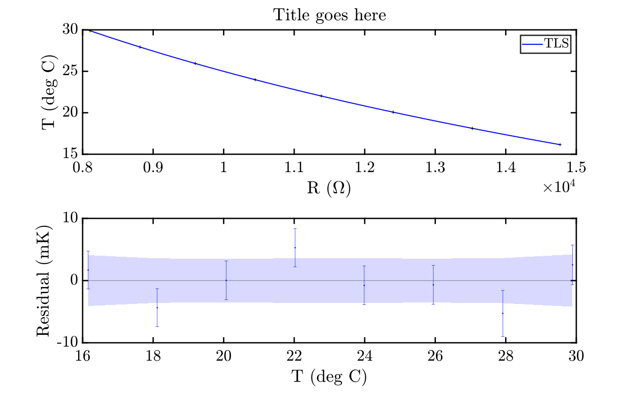
Here are those quantities applied to a representative thermistor calibration with the Steinhart–Hart model. The fit band from (3.2) is narrowest near the center of the calibration range and widens toward the edges; the total calibration uncertainty from (3.9) adds the propagated measurement uncertainty in the new resistance reading in quadrature.
4 LinearRegression: MATLAB and Python implementations
I keep two implementations of the WLS and TLS estimators derived above: LinearRegression.m in MATLAB and linear_regression.py in Python. Both build the design matrix automatically from a symbolic model string and compute the full uncertainty budget of Section 3. Both live at github.com/cjcrowley/curve-fitting, together with runnable examples and a test suite.
The Python version began as a direct port of the MATLAB one, and the two produce the same numbers: same estimator, same covariance, same $\max(1,\tilde{\chi}^2)$ inflation rule. They differ in one respect only. MATLAB draws the diagnostic figure from inside the fit call, whereas in Python the plot is a separate public function and the plotting options moved with it — so the two option lists are not interchangeable.
4.1 Architecture
Each implementation is one public entry point plus a set of subfunctions. The plotting routine is where they part: in MATLAB it's a private subfunction called from inside the fit, in Python a public module-level function called separately — so a figure can be regenerated from a stored result without re-running the fit.
| Role | MATLAB name | Python name | MATLAB | Python |
|---|---|---|---|---|
| Argument parsing, NaN removal, solver, uncertainty budget | LinearRegression | linear_regression | public | public |
| Symbolic differentiation → $\mathbf{X}$, $\mathbf{U}$ | build_design_matrix | _build_design_matrix | private | private |
| Formatted console output | print_summary | _print_summary | private | private |
| Two-panel diagnostic figure | make_plot | make_plot | private | public |
The top-level execution flow is identical in both:
- Inputs — $x$, $y$, $u_y$, optionally $u_x$, plus the model string, parameter names, and options.
- Dispatch — if the fourth argument is a string, the call is WLS; if it is numeric, the call is TLS.
- Clean — remove rows containing NaN.
- Build —
build_design_matrixreturns $\mathbf{X}$ and $\mathbf{U}$. - Solve — WLS in closed form, or TLS by iteratively reweighted least squares.
- Budget — compute $\mathrm{Cov}$, $\tilde{\chi}^2$, $w_\mathrm{rms}$, $u_\mathrm{total}$ under both options, and $\bar{u}$.
- Pack — return a struct (MATLAB) or dataclass (Python).
- Report — optionally print the summary. MATLAB also draws the figure here; Python leaves that to a separate
make_plotcall.
4.2 Design matrix construction
Both implementations build $\mathbf{X}$ and $\mathbf{U}$ analytically from the model string by symbolic differentiation — MATLAB through the Symbolic Math Toolbox (syms, diff, matlabFunction), Python through SymPy (sympy.Symbol, sympy.diff, sympy.lambdify). For each parameter $\beta_k$,
$$\begin{aligned} X_{ik} &= \left.\frac{\partial f}{\partial \beta_k}\right|_{x_i}, \\[6pt] U_{ik} &= \left|\frac{\partial^2 f}{\partial \beta_k\,\partial x}\right|_{x_i} u(x_i), \end{aligned}$$
the second being the GUM first-order propagation behind (2.8). No numerical differencing anywhere; both derivatives are exact.
Model strings use ordinary mathematical notation with x as the independent variable. MATLAB uses ^ for exponentiation; Python accepts both ^ and **, silently converting ^ to ** before parsing. The same model string therefore works in both languages:
modelStr = 'A + B*log(x) + D*(log(x))^3';
params = ["A", "B", "D"];model_str = 'A + B*log(x) + D*(log(x))^3' # ^ auto-converted to **
params = ['A', 'B', 'D']4.3 The iterative TLS solver
The TLS solver is iteratively reweighted least squares, selected automatically when the fourth argument is numeric (MATLAB) or is not a string (Python). At each iteration the effective variance (2.8) is recomputed from the current $\hat{\vec{\beta}}$, the weight matrix is updated, and a standard WLS solve is performed. Convergence is declared when
$$\left\|\hat{\vec{\beta}}^{(k+1)} - \hat{\vec{\beta}}^{(k)}\right\| < \varepsilon_{\mathrm{tol}}\left(1 + \left\|\hat{\vec{\beta}}^{(k)}\right\|\right), \qquad \varepsilon_{\mathrm{tol}} = 10^{-10}\ \text{(default)}.$$
If the iteration cap is reached without convergence, a warning is issued and the final iterate is returned. The initial guess defaults to the ordinary least-squares solution; a custom starting point can be supplied through the beta0 option.
4.4 The uncertainty budget
Following Section 3.3, both scatter-handling options are computed and stored side by side in the output, so the appropriate one can be chosen after the fact:
| Field | Formula | When to use |
|---|---|---|
uTotal_chi2scaled | $\sqrt{\vec{x}_i^\mathsf{T}\mathrm{Cov}_\mathrm{inf}\,\vec{x}_i}$ | $\tilde{\chi}^2 \gg 1$, scatter from underestimated $u$ |
uTotal_wrmsAdded | $\sqrt{u_{\hat{y}_i}^2 + w_\mathrm{rms}^2}$ | Genuine independent noise floor |
uBar_chi2scaled | (3.10), Option A | Single reportable number |
uBar_wrmsAdded | (3.10), Option B | Single reportable number |
These field names, and their contents, are identical in both implementations. covBeta_inf in particular follows the inflate-only rule (3.6) in both: the bands widen when the residuals exceed the uncertainty model, hold at $\mathrm{Cov}(\hat{\vec{\beta}})$ when they don't, and are never shrunk below what the input uncertainties support.
In MATLAB, do not pass covBeta_inf to the plot while also setting includeScatter to true — that double-counts the scatter. Python's plot takes the result object and picks the bands itself, so the conflict can't arise.
4.5 Display-unit conversion
An optional transform function $g(v)$ maps fit-space quantities into physical display units before printing and plotting. The local Jacobian comes from a relative-step finite difference,
$$g'(v_i) \approx \frac{g\!\left(v_i(1+\varepsilon)\right) - g(v_i)}{v_i\,\varepsilon}, \qquad \varepsilon = 10^{-6},$$
giving $u_\mathrm{display} = |g'(v_i)|\,u_\mathrm{fit\text{-}space}$. The relative step keeps the conditioning good regardless of the magnitude of $v_i$.
4.6 MATLAB interface
Requires MATLAB with the Symbolic Math Toolbox. The solver is chosen by inspecting the type of the fourth argument — a string means WLS, numeric means TLS.
% WLS (no x-uncertainty)
result = LinearRegression(x, y, uY, modelStr, params, Name, Value, ...)
% TLS (with x-uncertainty)
result = LinearRegression(x, y, uX, uY, modelStr, params, Name, Value, ...)| Name | Default | Description |
|---|---|---|
tol | 1e-10 | TLS convergence tolerance |
maxIter | 1000 | TLS maximum iterations |
beta0 | OLS | TLS initial guess ($p\times 1$) |
printSummary | true | Print the coefficient table and $\bar{u}$ to the console |
makePlot | true | Generate the two-panel diagnostic figure |
transformFcn | @(v)v | Fit-space → display-unit mapping |
displayUnit | '' | Unit label for the display axis |
residScale | 1 | Residual multiplier (e.g. 1000 for milli-units) |
residUnit | '' | Residual axis unit label |
xLabel | 'x' | Top-panel $x$-axis label |
yLabel | 'y' | Top-panel $y$-axis label |
xBotLabel | yLabel | Bottom-panel $x$-axis label |
plotTitle | '' | Figure title |
nGrid | 200 | Points in the dense fit curve |
xTopData | $x$ | Override the top-panel $x$-axis data |
xBotData | $y_\mathrm{disp}$ | Override the bottom-panel $x$-axis data |
includeScatter | true | Add $w_\mathrm{rms}$ to the CI bands (Option B); set false for Option A |
| Field | Size | Description |
|---|---|---|
beta | $p\times 1$ | $\hat{\vec{\beta}}$ |
uBeta | $p\times 1$ | $u(\hat{\beta}_j)$ from covBeta |
uBeta_inf | $p\times 1$ | $u(\hat{\beta}_j)$ from covBeta_inf |
covBeta | $p\times p$ | Covariance, input-$u$ based, (2.12) |
covBeta_inf | $p\times p$ | $\tilde{\chi}^2$-inflated covariance |
chi2r | scalar | $\tilde{\chi}^2$ |
wrms | scalar | $w_\mathrm{rms}$, in fit-space units |
uFit | $n\times 1$ | $u_{\hat{y}_i}$ from covBeta, (3.2) |
uFit_inf | $n\times 1$ | $u_{\hat{y}_i}$ from covBeta_inf |
uTotal_chi2scaled | $n\times 1$ | Per-point $u$, Option A |
uTotal_wrmsAdded | $n\times 1$ | Per-point $u$, Option B |
uBar_chi2scaled | scalar | $\bar{u}$ summary, Option A (fit space) |
uBar_wrmsAdded | scalar | $\bar{u}$ summary, Option B (fit space) |
uEff | $n\times 1$ | $u_{\mathrm{eff},i}$ |
X, uX | $n\times p$ | Design matrix and its uncertainty |
Xhat | $n\times p$ | Corrected design matrix (TLS; equals $\mathbf{X}$ for WLS) |
x_valid, y_valid | $n\times 1$ | Data after NaN removal |
method | string | 'WLS' or 'TLS' |
modelStr | string | Model string as passed |
params | string array | Parameter names as passed |
n, p | scalar | Observations used; parameters |
4.7 Python interface
pip install numpy sympy # required
pip install matplotlib # optional: only needed for make_plotmatplotlib is imported lazily inside make_plot, which also forces the Agg backend so no window ever opens. The module imports cleanly without it, and make_plot returns None rather than raising if it's missing.
The dispatch logic matches MATLAB: the fourth argument is inspected at runtime and the solver chosen accordingly. Unlike MATLAB, the fit does not draw a figure — call make_plot separately.
from linear_regression import linear_regression, make_plot
# WLS (no x-uncertainty)
result = linear_regression(x, y, uY, model_str, params, **kwargs)
# TLS (with x-uncertainty)
result = linear_regression(x, y, uX, uY, model_str, params, **kwargs)
# Plot, whenever you want, from a stored result
fig = make_plot(result, resid_scale=1000, resid_unit='mK')
fig.savefig('fit.png', dpi=150) # caller saves and closesAll options are keyword arguments rather than name–value pairs, in snake_case throughout.
| Keyword | Default | Description |
|---|---|---|
tol | 1e-10 | TLS convergence tolerance |
max_iter | 1000 | TLS maximum iterations |
beta0 | OLS | TLS initial guess (ndarray, $p\times 1$) |
print_summary | True | Print the coefficient table and $\bar{u}$ to the console |
transform_fcn | None | Fit-space → display-unit mapping (callable) |
display_unit | '' | Unit label for the display axis |
resid_scale | 1.0 | Residual multiplier (e.g. 1000 for milli-units) |
resid_unit | '' | Residual axis unit label |
x_label | 'x' | Label carried into the printed summary |
y_label | 'y' | Label carried into the printed summary |
plot_title | '' | Title carried into the printed summary |
All arguments to make_plot after result are keyword-only. It returns the matplotlib Figure, or None if matplotlib isn't installed; saving and closing it is the caller's job.
| Keyword | Default | Description |
|---|---|---|
transform_fcn | None | Fit-space → display-unit mapping (callable) |
resid_scale | 1.0 | Residual multiplier (e.g. 1000 for milli-units) |
resid_unit | '' | Residual axis unit label |
x_label | 'x' | Top-panel $x$-axis label |
y_label | 'y' | Top-panel $y$-axis label |
x_bot_label | '' | Bottom-panel $x$-axis label (defaults to y_label) |
plot_title | '' | Figure title |
n_grid | 200 | Points in the dense fit curve |
x_top_data | None | Override the top-panel $x$-axis data |
x_bot_data | None | Override the bottom-panel $x$-axis data |
k | 2.0 | Coverage factor for the plotted bands and error bars |
show_inflated | True | Also draw the $\tilde{\chi}^2$-inflated band over the non-inflated one; False draws only the latter |
floor_disp | 0.0 | Systematic floor added to the displayed bands |
Both bands are drawn at the same coverage factor $k$ and overlap semi-transparently, so the inflated and non-inflated intervals are visible at once. $k=1$ is deliberately never used by this figure — the bands in the thermistor figure above came from the MATLAB routine, which plots at $k=1$.
The function returns a RegressionResult dataclass. Every field supports dot access (result.beta, result.chi2r), matching the MATLAB struct syntax, and the field names are identical to the MATLAB struct with one exception: modelStr becomes model_str.
4.8 Examples
Steinhart–Hart thermistor calibration
The Steinhart–Hart model relates thermistor resistance $R$ to temperature $T$ through $1/T = A + B\ln R + D(\ln R)^3$, so the fit runs in $1/T$ space and a transform function converts the result back to degrees Celsius for display. The TLS call additionally propagates the resistance uncertainty $u(R)$ through the design matrix.
% --- Data ---
R = [...]; % resistance [Ohm]
T = [...] + 273.15; % temperature [K]
uR = [...]; % standard uncertainty in R [Ohm]
uT = [...]; % standard uncertainty in T [K]
uOneOverT = uT ./ T.^2; % propagated uncertainty in 1/T [1/K]
% --- Model ---
modelStr = 'A + B*log(x) + D*(log(x))^3';
params = ["A", "B", "D"];
% WLS: uncertainty in y (1/T) only
wls = LinearRegression(R, 1./T, uOneOverT, modelStr, params, ...
'transformFcn', @(v) 1./v - 273.15, ...
'xLabel', 'R ($\Omega$)', 'yLabel', 'T ($^\circ$C)', ...
'residScale', 1000, 'residUnit', 'mK', ...
'plotTitle', 'Steinhart--Hart WLS');
% TLS: uncertainty in both R and 1/T
tls = LinearRegression(R, 1./T, uR, uOneOverT, modelStr, params, ...
'transformFcn', @(v) 1./v - 273.15, ...
'xLabel', 'R ($\Omega$)', 'yLabel', 'T ($^\circ$C)', ...
'residScale', 1000, 'residUnit', 'mK', ...
'plotTitle', 'Steinhart--Hart TLS');
% --- Access results ---
fprintf('WLS A = %.4e +/- %.4e\n', wls.beta(1), wls.uBeta(1));
fprintf('WLS chi2r = %.4f\n', wls.chi2r);
fprintf('WLS uBar (Option B) = %.2f mK\n', wls.uBar_wrmsAdded * 1000);import numpy as np
from linear_regression import linear_regression, make_plot
# --- Data ---
R = np.array([...]) # resistance [Ohm]
T = np.array([...]) + 273.15 # temperature [K]
uR = np.array([...]) # standard uncertainty in R [Ohm]
uT = np.array([...]) # standard uncertainty in T [K]
uOneOverT = uT / T**2 # propagated uncertainty in 1/T [1/K]
# --- Model ---
model_str = 'A + B*log(x) + D*(log(x))^3'  # ^ auto-converted to **
params    = ['A', 'B', 'D']
# WLS: uncertainty in y (1/T) only
wls = linear_regression(
R, 1.0/T, uOneOverT, model_str, params,
transform_fcn = lambda v: 1.0/v - 273.15,
x_label = r'R ($\Omega$)',
y_label = r'T ($^\circ$C)',
resid_scale = 1000,
resid_unit = 'mK',
plot_title = 'Steinhart-Hart WLS')
# TLS: uncertainty in both R and 1/T
tls = linear_regression(
R, 1.0/T, uR, uOneOverT, model_str, params,
transform_fcn = lambda v: 1.0/v - 273.15,
x_label = r'R ($\Omega$)',
y_label = r'T ($^\circ$C)',
resid_scale = 1000,
resid_unit = 'mK',
plot_title = 'Steinhart-Hart TLS')
# --- Access results ---
print(f"WLS A = {wls.beta[0]:.4e} +/- {wls.uBeta[0]:.4e}")
print(f"WLS chi2r = {wls.chi2r:.4f}")
print(f"WLS uBar (Option B) = {wls.uBar_wrmsAdded * 1000:.2f} mK")
# --- Figures (a separate call in Python) ---
for res, name in ((wls, 'wls'), (tls, 'tls')):
fig = make_plot(
res,
transform_fcn = lambda v: 1.0/v - 273.15,
x_label = r'R ($\Omega$)',
y_label = r'T ($^\circ$C)',
resid_scale = 1000,
resid_unit = 'mK',
plot_title = f'Steinhart-Hart {name.upper()}')
fig.savefig(f'steinhart_hart_{name}.png', dpi=150)Quadratic polynomial
A plain quadratic $y = A + Bx + Cx^2$ with uniform $y$-uncertainties. No transform function, because fit space and display space are the same.
% --- Model ---
modelStr = 'A + B*x + C*x^2';
params   = ["A", "B", "C"];

% WLS
result = LinearRegression(x, y, uY, modelStr, params, ...
    'xLabel', 'x', 'yLabel', 'y', ...
    'plotTitle', 'Quadratic fit');

% --- Access results ---
fprintf('A = %.4g,  B = %.4g,  C = %.4g\n', ...
    result.beta(1), result.beta(2), result.beta(3));
fprintf('Reduced chi-squared: %.4f\n', result.chi2r);# --- Model ---
model_str = 'A + B*x + C*x**2' # or 'A + B*x + C*x^2' -- both work
params = ['A', 'B', 'C']
# WLS
result = linear_regression(x, y, uY, model_str, params,
x_label = 'x',
y_label = 'y',
plot_title = 'Quadratic fit')
# --- Access results ---
A, B, C = result.beta
print(f"A = {A:.4g}, B = {B:.4g}, C = {C:.4g}")
print(f"Reduced chi-squared: {result.chi2r:.4f}")References
- [1] P. R. Bevington and D. K. Robinson, Data Reduction and Error Analysis for the Physical Sciences, 3rd ed. Boston: McGraw-Hill, 2003.
- [2] Joint Committee for Guides in Metrology, Evaluation of Measurement Data — Guide to the Expression of Uncertainty in Measurement, JCGM 100:2008 (GUM 1995 with minor corrections). BIPM
- [3] B. N. Taylor and C. E. Kuyatt, Guidelines for Evaluating and Expressing the Uncertainty of NIST Measurement Results, NIST Technical Note 1297. Gaithersburg, MD, 1994. NIST